Investigating the effect of noise on the area uncertainty quantification

%load_ext autoreload
%autoreload 2

import numpy as np
import pandas as pd
import arviz as az
import pymc as pm
from pathlib import Path
from peak_performance import pipeline as pl, models, plots
from matplotlib import pyplot as plt

Load and inspect raw intensity data

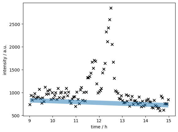
timeseries = np.load(Path(r"..\example\A2t2R1Part1_132_85.9_86.1.npy"))
time = timeseries[0]
ints = timeseries[1]

def guess_noise(intensity):
    n = len(intensity)
    ifrom = int(np.ceil(0.15 * n))
    ito = int(np.floor(0.85 * n))
    start_ints = intensity[:ifrom]
    end_ints = intensity[ito:]
    return np.std([*(start_ints - np.mean(start_ints)), *(end_ints - np.mean(end_ints))])

fig, ax = plt.subplots()
ax.scatter(timeseries[0], timeseries[1], marker="x", color="black")
slope, intercept, noise = models.initial_guesses(time, ints)
ax.fill_between(
    time,
    slope * time + intercept - noise / 2,
    slope * time + intercept + noise / 2,
    alpha=0.5
)
ax.set(
    xlabel="time / h",
    ylabel="intensity / a.u.",
)
plt.show()

Define a peak model

pmodel = models.define_model_double_normal(
    time=timeseries[0],
    intensity=timeseries[1]
)
pmodel.to_graphviz()

c:\Users\osthege\AppData\Local\mambaforge\envs\pepe\Lib\site-packages\pymc\data.py:273: FutureWarning: ConstantData is deprecated. All Data variables are now mutable. Use Data instead.
  warnings.warn(

Fix the noise settings using pm.do

pm.do(pmodel, {"noise_width_guess": 100}).to_graphviz()

Sample the models with fixed noise

sigma_idatas = {}
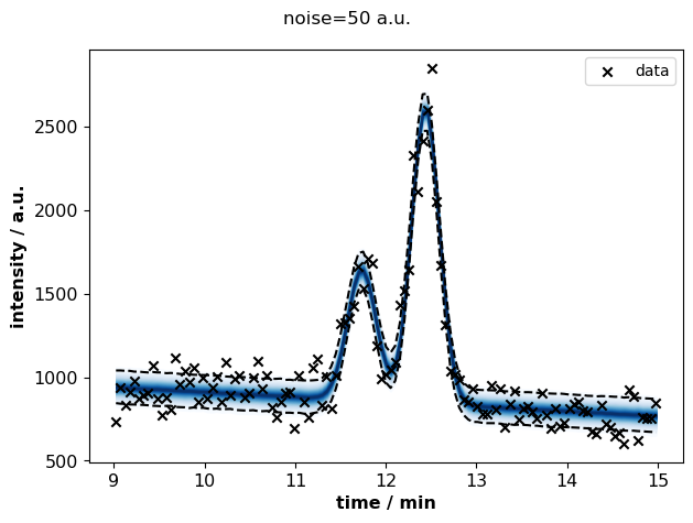
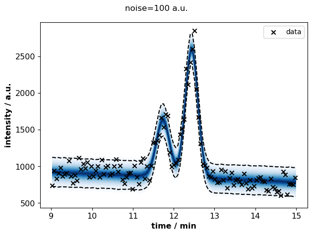
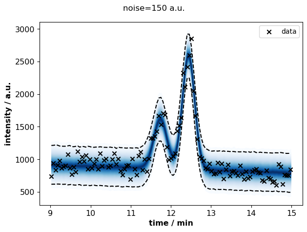
for s in [50, 100, 150, 200, 300, 400, 500]:
    spmodel = pm.do(pmodel, {"noise": s})
    sigma_idatas[s] = pl.sampling(spmodel, tune=6_000, draws=2000)
    sigma_idatas[s] = pl.posterior_predictive_sampling(spmodel, sigma_idatas[s])

Sampling: [L, baseline_intercept, baseline_slope, height, meanmean, separation, std]

100.00% [32000/32000 00:02<00:00 Sampling chains: 0, Divergences: 0]

Sampling: [L]

Sampling: [L, baseline_intercept, baseline_slope, height, meanmean, separation, std]

100.00% [32000/32000 00:03<00:00 Sampling chains: 0, Divergences: 0]

Sampling: [L]

Sampling: [L, baseline_intercept, baseline_slope, height, meanmean, separation, std]

100.00% [32000/32000 00:03<00:00 Sampling chains: 0, Divergences: 0]

Sampling: [L]

Sampling: [L, baseline_intercept, baseline_slope, height, meanmean, separation, std]

100.00% [32000/32000 00:02<00:00 Sampling chains: 0, Divergences: 0]

Sampling: [L]

Sampling: [L, baseline_intercept, baseline_slope, height, meanmean, separation, std]

100.00% [32000/32000 00:03<00:00 Sampling chains: 0, Divergences: 0]

Sampling: [L]

Sampling: [L, baseline_intercept, baseline_slope, height, meanmean, separation, std]

100.00% [32000/32000 00:03<00:00 Sampling chains: 0, Divergences: 0]

Sampling: [L]

Sampling: [L, baseline_intercept, baseline_slope, height, meanmean, separation, std]

100.00% [32000/32000 00:02<00:00 Sampling chains: 0, Divergences: 1]

Sampling: [L]

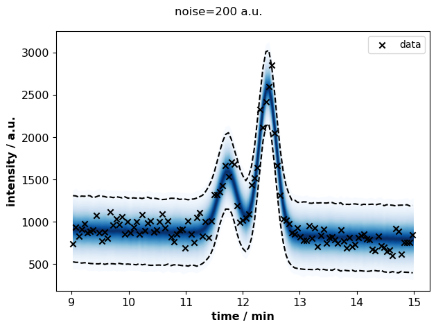
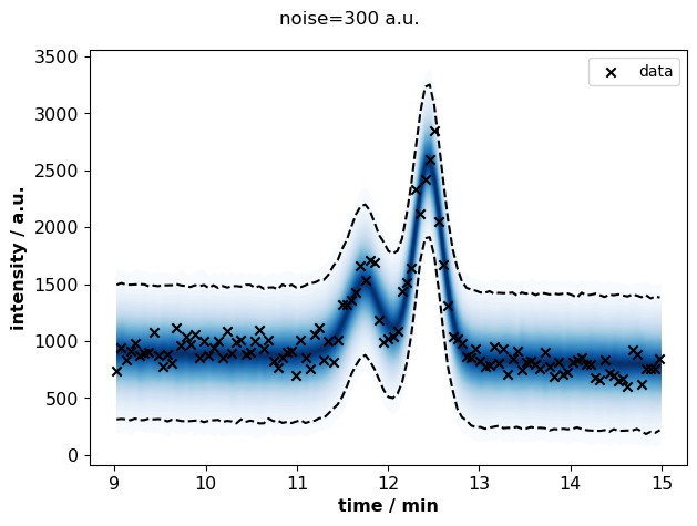
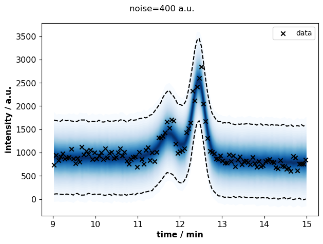
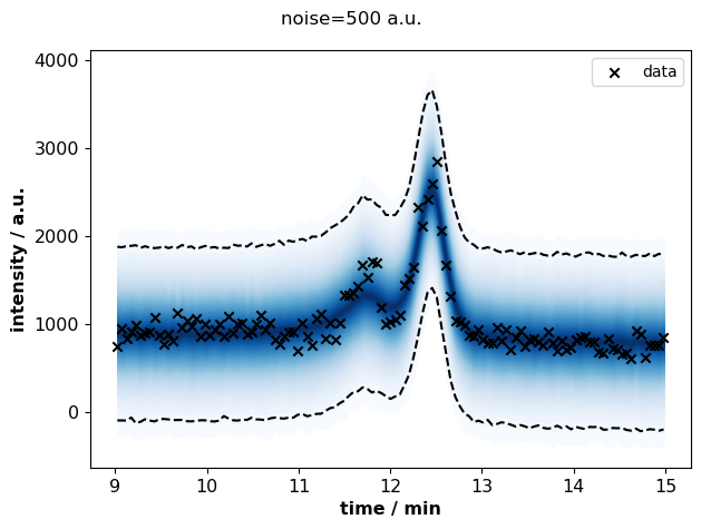
for s, idata in sigma_idatas.items():
    plots.plot_posterior_predictive(
        identifier="peak_fit",
        time=idata.constant_data.time.values,
        intensity=idata.constant_data.intensity.values,
        path=None,
        idata=idata,
        discarded=False,
    )
    fig = plt.gcf()
    fig.suptitle(f"noise={s} a.u.")
    fig.tight_layout()
    plt.show()

summary = pd.concat([
    az.summary(idata, var_names=["area"])
    for s, idata in sigma_idatas.items()
], keys=sigma_idatas, names=["noise", "var_name"])
summary

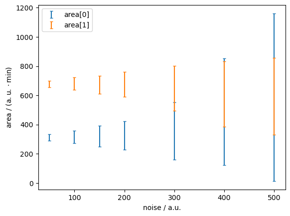
		mean	sd	hdi_3%	hdi_97%	mcse_mean	mcse_sd	ess_bulk	ess_tail	r_hat
noise	var_name
50	area[0]	313.351	11.665	291.073	334.905	0.109	0.077	11348.0	6043.0	1.0
	area[1]	678.536	11.291	656.315	698.359	0.105	0.075	11806.0	5822.0	1.0
100	area[0]	316.106	23.420	272.294	359.828	0.215	0.153	11865.0	6763.0	1.0
	area[1]	675.603	22.394	636.958	722.187	0.200	0.142	12404.0	5899.0	1.0
150	area[0]	319.884	37.831	249.006	391.667	0.369	0.263	10519.0	6268.0	1.0
	area[1]	673.569	32.766	611.630	734.258	0.301	0.213	11899.0	6263.0	1.0
200	area[0]	324.587	52.400	229.037	423.322	0.585	0.433	8537.0	5144.0	1.0
	area[1]	670.918	44.970	592.101	761.562	0.463	0.327	9483.0	5651.0	1.0
300	area[0]	358.377	125.401	160.648	551.351	2.581	2.006	3855.0	2160.0	1.0
	area[1]	650.773	81.505	493.518	801.641	1.647	1.165	2905.0	1754.0	1.0
400	area[0]	435.775	233.185	123.857	853.499	4.999	3.535	2735.0	3092.0	1.0
	area[1]	614.937	117.477	386.018	833.273	2.432	1.720	2418.0	2722.0	1.0
500	area[0]	540.067	369.859	14.128	1160.742	8.399	6.922	2429.0	2371.0	1.0
	area[1]	589.281	142.407	329.538	856.490	2.730	1.931	2686.0	3486.0	1.0

fig, ax = plt.subplots()

for vname, df in summary.reset_index().groupby("var_name"):
    ax.errorbar(
        df["noise"],
        y=df["mean"],
        yerr=[
            df["mean"] - df["hdi_3%"],
            df["hdi_97%"] - df["mean"],
        ],
        label=vname,
        ls="none",
        capsize=2,
    )
ax.legend()
ax.set(
    xlabel="noise / a.u.",
    ylabel="$\mathrm{area\ /\ (a.u. \cdot min)}$"
)
plt.show()

Conclusion

• At high noise (>200 a.u.), the uncertainty about peak areas increases.

• In this case, the model fits a noise of ~115 a.u. so that’s well below the critical level.

%load_ext watermark
%watermark -idu

The watermark extension is already loaded. To reload it, use:
  %reload_ext watermark
Last updated: 2024-05-11T14:43:08.623240+02:00