Example 1: Build a pipeline using PeakPerformance’s convenience functions#

import pandas
import numpy as np
import arviz as az
from pathlib import Path
from peak_performance import pipeline as pl

User information#

First, store the path to a folder containing only the raw data you want to analyze in the path_raw_data variable.
Then, store the path to the directory containing the Excel file Template.xlsx from PeakPerformance in the path_template variable. You can download the file directly from GitHub or clone the PeakPerformance repository locally.
You can use a string with a preceding r so that the backslashes are recognized correctly or the Path method from the pathlib package for an OS-independent alternative.

For this example, the general paths within the PeakPerformance repository have already been formulated below (it is recommended to clone the repository on your local machine).

# specify the absolute path to the raw data files (as a str or a Path object), e.g. to the provided example files

path_raw_data = Path("..") / "example"
path_template = Path("..")

The first step of the process is always the prepare_model_selection() function. Its job is to prepare and partly fill out an Excel file called Template.xlsx which serves as the input for user data and is copied into the directory stored in the path_raw_data variable. Conveniently, the function only needs the two paths you defined above.

pl.prepare_model_selection(path_raw_data, path_template)

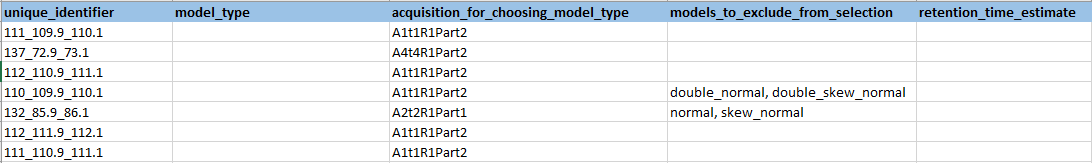
Now, navigate to the directory stored in path_raw_data and open Template.xlsx. Read the explanations and fill out the sheets accordingly. Then, save and close the Excel file (not closing it leads to a permission error when executing the next method).

The next step depends on what information you entered into Template.xlsx. If you specified a model type for peak fitting for every unique_identifier, then you can skip the automated model selection described in the next section. If you left the model type open for at least one unique_identifier, then go ahead with the automated model selection.

Automated model selection (optional)#

The intended standard workflow involves an automated selection of the model or distribution used for peak fitting. This is performed based on a representative peak for every target analyte (or unique_identifier as they are referred to in Template.xlsx). For each of these, an information criterion is calculated based on which the models are ranked and the best model for any given target is selected. Finally, Template.xlsx is updated with these selected models wherever no model was specified by the user.

This step may take a while since every file in question is fit with each of the models and the number of tuning samples is higher than usual so the sampling time per model is additionally increased.

The returned model_dict is a dictionary with the unique_identifiers as keys and the selected models as values.
The returned result is a DataFrame with all rankings from the model selection process.

When using the example data, you can use the following settings. It is, however, highly recommended to checkout example notebook 3 to test the model selection instead, since a) example 3 features several peaks per analyte which represents a more realistic case and b) most of the data in this example is noise and will be filtered out, anyways.

result, model_dict = pl.model_selection(path_raw_data)

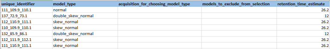
In case you left Template.xlsx open and received a UserWarning to that effect, just close it now and execute the subsequent cell to update Template.xlsx with the results of the model selection. Otherwise, skip the next cell.

df_signals = pandas.read_excel(Path(path_raw_data) / "Template.xlsx", sheet_name="signals")
pl.selected_models_to_template(path_raw_data, df_signals, model_dict)

Pipeline#

When every unique_identifier has been matched with a model type, it is time to start the actual peak fitting pipeline. This is once again done with just one simple command which needs the already defined path_raw_data variable. Additionally, the user has to supply the data format of the raw data files. The example files are “.npy” files but others are acceptable as long as they follow PeakPerformance’s standardized naming scheme and contain the correctly formatted data.

When triggering the pipeline, a folder for the results named after the current date and time will be created automatically in the directory with the raw data files. The path to this folder will be returned and stored in the results variable.

When using the example data, you can use the following settings:

results = pl.pipeline(
    path_raw_data = path_raw_data,
    raw_data_file_format = ".npy",
)

results

Data analysis#

Since the inference data objects for all signals were saved in the path stored in results, you can open any one you are interested in with the command idata = az.from_netcdf().
These objects contain not only the timeseries of the particular signal but also samples from the prior predictive, posterior, and posterior predictive sampling.
This allows you to explore the data in detail and/or build your own plots aside from the ones featured in PeakPerformance.

It is highly recommended to check the documentations for PyMC and ArviZ to get information and inspiration for this purpose.

# open an inference data object
idata = az.from_netcdf(results / "A1t1R1Part2_110_109.9_110.1.nc")
idata

arviz.InferenceData

posterior
posterior_predictive
sample_stats
prior
prior_predictive
observed_data
constant_data
warmup_posterior
warmup_sample_stats

# store the summary in the DataFrame az_summary
az_summary = az.summary(idata)
az_summary

	mean	sd	hdi_3%	hdi_97%	mcse_mean	mcse_sd	ess_bulk	ess_tail	r_hat
baseline_intercept	-44.003	7.227	-57.478	-30.260	0.079	0.057	8290.0	6088.0	1.0
baseline_slope	6.659	0.514	5.672	7.616	0.007	0.005	5471.0	5696.0	1.0
noise_log__	4.645	0.073	4.510	4.785	0.001	0.001	9311.0	5961.0	1.0
mean	25.949	0.013	25.926	25.975	0.000	0.000	2650.0	3786.0	1.0
std_log__	-0.644	0.042	-0.727	-0.568	0.001	0.001	2429.0	2921.0	1.0
...	...	...	...	...	...	...	...	...	...
y[94]	147.639	13.291	123.255	172.644	0.168	0.119	6287.0	6354.0	1.0
y[95]	147.941	13.311	123.565	173.030	0.168	0.119	6280.0	6251.0	1.0
y[96]	148.243	13.332	123.833	173.360	0.168	0.119	6274.0	6251.0	1.0
y[97]	148.545	13.352	124.101	173.711	0.168	0.119	6268.0	6251.0	1.0
y[98]	148.848	13.373	124.369	174.067	0.169	0.120	6264.0	6251.0	1.0

217 rows × 9 columns

Example 1: Build a pipeline using PeakPerformance’s convenience functions

Contents

Example 1: Build a pipeline using PeakPerformance’s convenience functions#

User information#

Automated model selection (optional)#

Pipeline#

Data analysis#